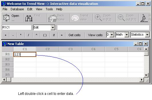
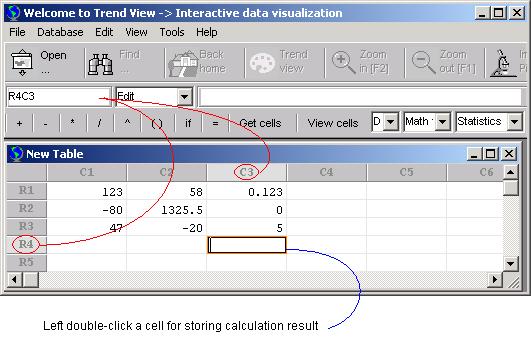
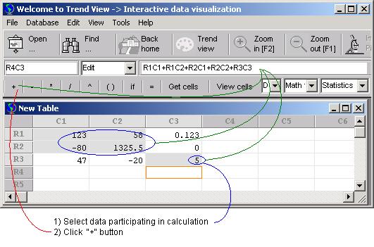
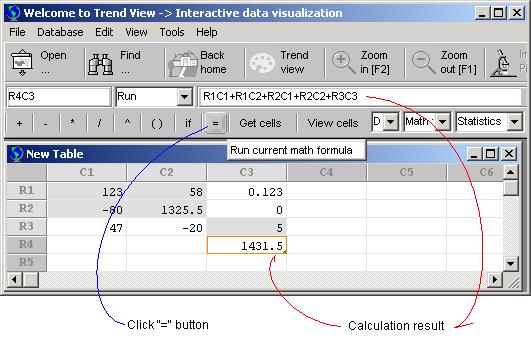
InforShell


Trend View

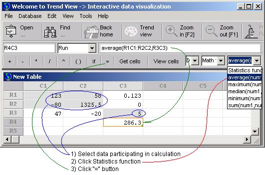
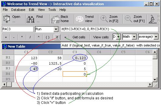
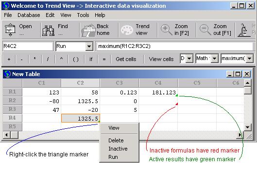
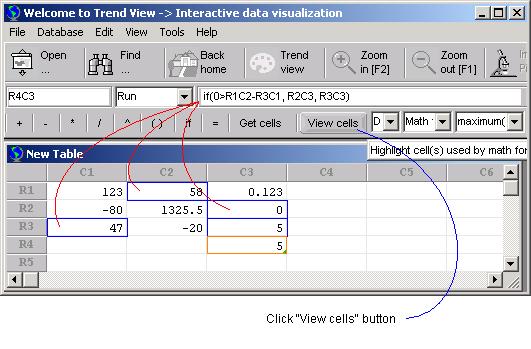
Math Formula and Supporting Features
- Operation Overview


Data & Math Formula Entry

  • Opening Trend View Spreadsheet
  • Entering Data
  • Specifying Calculation Output Cell
  • Specifying Input Cells and Composing Formula
  • Displaying Calculation Result
  • Using Math or Statistics Functions
  • Using "If( )" Condition
  • Distinction Between Addition and Summation Functions
  • Using "count_if( )" Functions
  • Using "sum_if( )" Functions


  • Supporting Features

  • Formula Status and Red/Green Corner Marker
  • Deleting Calculation Result
  • Transferring Formula to Multiple Rows/Columns
  • Modifying Input Data
  • Viewing Input Cells of Current Result
  • Locking and Releasing a Row/Column's Position
  • Adjusting Cell Size and Text Wrapping
  • Saving Trend View Spreadsheet File


  • Opening Trend View Spreadsheet

  • Double-click TrendView.exe from the folder it is stored.
  • Under "File", select "New" to open a blank spreadsheet or select "Open" to access an existing spreadsheet file.
  • Entering Data

  • Double-click a cell using the left mouse button
  • Enter data using the keyboard.
  • Press the Tab key, cursor will move to the cell to the right;
  • Press the Enter key, cursor will move to the cell below;
  • Each cell can store a maximum of 500 letters or numbers.

  • Figure 1: Entering Data

    Return to Top


    Specifying Calculation Output Cell

  • Choose a cell to store the calculation result, and double-click with the left mouse button
  • The selected cell's reference will be visible in the spreadsheet's upper left Target Cell Box.

  • Figure 2: Specifying calculation output cell

    Return to Top


    Specifying Input Cells and Composing Formula

    Simple math operators provided in the spreadsheet include: + (Addition), - (Subtraction), * (Multiplication), / (Division), ^ (Power), ( ) , if

    Applying a single math operator (For example, Addition)

  • Left-click to select (holding down "Ctrl" key to select multiple) the cells containing input data for the current calculation.
  • Click "+" button on the Tool Bar
  • Selected cells and addition operator will automatically be written into the "User Math Formula Edit Box"
  • Applying multiple operators

  • Left-click to select (holding down "Ctrl" key to select multiple) the cells containing input data for the current calculation.
  • Click "Get cells" button on the Tool Bar
  • Selected cells and question mark delimiter will automatically be written into the "User Math Formula Edit Box", e.g. R1C1?R1C2?R2C1?R2C2?R3C3
  • Directly edit the formula as needed, e.g.: (R1C1+R1C2-(R2C1+R2C2))*R3C3

  • Figure 3: Addition calculation

    Return to Top


    Displaying Calculation Result

    Using the same addition example above, after "R1C1+R1C2+R2C1+R2C2+R3C3" is shown in the "User Math Formula Edit Box"

  • Click "=" button on the Tool Bar or press "Enter" on the keyboard
  • Calculation result (including formula) will be written into the target cell.

  • Figure 4: Displaying calculation result

    Return to Top


    Using Math or Statistics Functions

    For example, finding the average of a dataset

  • Left-click while holding down "Ctrl" key to select all the cells to be averaged.
  • Under the "Statistics Functions" drop down menu on the Tool Bar, select "average"
  • Selected cells and function will automatically be written into the "User Math Formula Edit Box"
  • Click "=" button on the Tool Bar or press "Enter" on the keyboard
  • Calculation result (including formula) will be written into the target cell.
  • Functions provided in the spreadsheet include

  • 16 math functions, including: cos( ), log( ), exp( ), pow( ), sin( );
  • 5 statistics functions, including: maximum( ), average( ), sum( ), etc;
  • Functions can be used as argument to other functions.
  • Statistics function input syntax
    Reference to a range of cells is supported via the colon symbol and references of the upper-left and lower-right corner cells. In this example "R1C1:R2C2". Multiple ranges can be used for calculation, separated by a comma. In this example "R1C1:R2C2,R3C3"


    Figure 5: Finding the average

    Return to Top


    Using "If( )" Condition

    The syntax for using the "if" function is: if (comparison condition, formula to evaluate when true, formula to evaluate when false). For example, to set the operation "if R1C3 - R3C1<0 is true, then output 0, other wise output result of R1C3 - R3C1", use the following steps:

  • Select output cell, e.g. double-click R4C3
  • Left-click to select (holding down "Ctrl" key to select multiple) the cells containing input data for the current calculation.
  • Click "if" button on the Tool Bar
  • Selected cells and function will automatically be written into the "User Math Formula Edit Box", e.g. if( R1C3?R3C1)
  • Edit the formula as needed, e.g. if(R1C3 - R3C1<0, 0, R1C3 - R3C1)
  • Click "=" button on the Tool Bar or press "Enter" on the keyboard
  • Calculation result (including formula) will be written into the target cell R4C3
  • Comparison condition syntax

  • A equal to B: A = B or A == B
  • A not equal to B: A != B or A <> B
  • A greater than B: A > B
  • A greater than or equal to B: A >= B or A => B
  • A less than B: A < B
  • A less than or equal to B: A <= B or A =< B

  • Figure 6: Using "if" condition

    "Or" operation
    For example, to set "If R1C2 - R3C1<0 Or R1C2 - R3C1>10 , then evaluate R2C3, otherwise evaluate R3C3", the "if" formula can be written as

  • if(R1C2 - R3C1<0, R2C3, if(R1C2 - R3C1>10, R2C3, R3C3 ) )
  • "And" operation
    For example, to set "If R1C2 - R3C1 not equal 0 and R1C2 - R3C1 not equal 10, then evaluate R2C3, otherwise evaluate R3C3", the "if" formula can be written as

  • if(R1C2 - R3C1<> 0, if(R1C2 - R3C1<>10, R2C3, R3C3 ), R3C3 )
  • Return to Top


    Distinction Between Addition and Summation Functions

    The addition and summation functions process input cells differently. If some input cells to the summation function contain text, these cells will be ignored. The addition (+) operator however, will generate an error when operand cells are not numeric.

    Return to Top


    Using "count_If( )"

    Syntax count_if( C1:Cn, "if")

    C1:Cn is the range of cells you want to evaluate. For example, C1:Cn can be written as R1C1:R1C4 or R1C1, R1C2, R1C3, R1C4.

    "if" is the criteria that defines which cells will be counted. It be a number or text, for example "=32", "29<=", "pencils" (double quotes are required) or a formula e.g. sin(R1C2). When searching for strings, the "*" can be used as wildcard.


    Example

    (1) Suppose R1C1:R1C4 contain the following data: 100, 200, 300, 400.
    count_if(R1C1:R1C4,">=200") equals 3
    count_if(R1C1:R1C4,"200<=") equals 3

    (2) Suppose R1C1:R1C4 contain the following text: aaa, abc, ccc, ddd.
    count_if(R1C1:R1C4,"ccc") equals 1
    count_if(R1C1:R1C4,"a*") equals 2

    (3) Suppose R1C1:R1C4 contain the following data: 100, 200, 300, 400.
    count_if(R1C1,R1C2,R1C3,R1C4,"!=200") equals 3

    Return to Top


    Using "sum_If( )"

    Syntax sum_if( C1:Cn, "if", N1:Nn)

    C1:Cn is the range of cells you want to evaluate. For example, C1:Cn can be written as R1C1:R1C4 or R1C1, R1C2, R1C3, R1C4.

    "if" is the criteria that defines which cells will be counted. It can be a number or text, for example "=32", "29<=", "pencils" (double quotes are required) or a formula e.g. sin(R1C2). When searching for strings, the "*" can be used as wildcard.

    N1:Nn is the range of cells to sum. For example, N1:Nn can be expressed as R1C1:R1C4 or R1C1, R1C2, R1C3, R1C4. The cells in N1:Nn are summed only if their corresponding cells in C1:Cn satisfy the "if" criteria.

    Note C1:Cn and N1:Nn should have the same notation (both comma delimited or both as a range).


    Example

    (1) Suppose R1C1:R1C4 contain the following data: 100, 200, 300, 400. R2C1:R2C4 contain the following data: 10, 40, 80, 70.
    sum_if(R1C1:R1C4,">=200",R2C1:R2C4) equals 190
    sum_if(R1C1:R1C4,"200<=",R2C1:R2C4) equals 190

    (2) Suppose R1C1:R1C4 contain the following text: aaa, abc, ccc, ddd. R2C1:R2C4 contain the following data: 7000, 10000, 21000, 28000.
    sum_if(R1C1:R1C4,"ccc",R2C1:R2C4) equals 21000
    sum_if(R1C1:R1C4,"a*",R2C1:R2C4) equals 17000

    (3) Suppose R1C1:R1C4 contain the following data: 100, 200, 300, 400. R2C1:R2C4 contain the following data: 10, 40, 80, 70.
    sum_if(R1C1,R1C2,R1C3,R1C4,"!=200",R2C1,R2C2,R2C3,R2C4) equals 160

    Return to Top


    Formula Status and Red/Green Corner Marker

    Formulas can be in either "active" or "inactive" state.

  • After entering the formula, clicking "=" button on the Tool Bar or pressing "Enter" on the keyboard will run the calculation and display result, the current formula will hence be in an active state. The output cell will indicate active state by showing a green triangle at its lower-right corner.
  • To only store a formula in a cell, but not perform the calculation - unused or incomplete formulas for example, users can select "Inactive" in the drop down menu left of the "User Math Formula Edit Box". Shifting Target Cell focus by double-clicking on a different cell while editing a formula will also change it to inactive state. Since no calculation result was generated, the output cell will be blank with a red triangle at its lower-right corner to indicate inactive state.
  • Right clicking the corner marker will open a pop-up menu for changing the formula's state.
  • Deleting Calculation Result

    Calculation result in a cell is deleted by deleting its formula.

  • Right click the green or red corner marker, on the pop-up menu select "Delete" to delete calculation result and formula of the target cell.

  • Figure 7: Formula state

    Return to Top


    Transferring Formula to Multiple Rows/Columns

    If in a spreadsheet, multiple rows/columns require the same formula, users can

  • Enter one instance of the formula manually in a cell.
  • Right-click the red/green corner marker and drag across several rows/columns to transfer the formula to other cells.
  • When the formula is transferred, the references of input cells involved in the calculation will update automatically according to the direction of transfer. If the formula requires modification, users will need to first modify the original formula, then repeat the above process of transferring the formula again.

    Modifying Input Data

  • When contents of cells participating in a formula are modified, the affected calculation results will update automatically;
  • All down-stream calculations will also be updated automatically.

  • Figure 8: Transferring formula to multiple rows/columns.

    Return to Top


    Viewing Input Cells of Current Result

    To view input cells to a calculation result, users can

  • Double-click the calculation output cell;
  • Click "View cells" button on the Tool Bar;
  • Cells participating in the calculation will be shown using a blue border.

  • Figure 9: Viewing input cells of calculation result

    Return to Top


    Locking and Releasing a Row/Column's Position

    If it is desirable to have a row or column's display position be fixed in the window (e.g. title row), and not shift when users are scrolling through the remaining cells, users can

  • Right-click the heading cell of this row/column to lock its position.
  • Right-click again (a locked row/column's heading cell) to release.

  • Figure 10: Locking title row's display position.

    Return to Top


    Adjusting Cell Size and Text Wrapping

    To adjust the height/width of a particular row/column, users can:

  • Left-click at the bottom/right edge of the row/column's heading cell, when the size adjustment cursor appears, adjust size by dragging the edge.
  • To enable text wrapping in a particular cell, increase the cell's row height using the method above.

  • Figure 11: Adjusting row/column size.

    Return to Top


    Saving Trend View Spreadsheet File

  • Trend View spreadsheets contain user entered formulas, data, text, and formatting (e.g. colors, font) information, which can be saved using the *.trv extension, e.g. "MyTable.trv".
  • Trend View spreadsheets can also be saved in text only (.txt) format, however formulas and formatting will not be preserved. The main use for a text only version is to enable other editors or spreadsheets to open the file and access saved data (e.g. Excel).
  • Return to Top